Variance based modelling
This vignette provides an introduction to variance-based modeling
using the admr package in R. We’ll cover the essential
steps to prepare your data, specify a pharmacokinetic model, fit the
model to aggregate data, and evaluate the results. We’ll compare the
results of using mean and variance only data to the full mean and
covariance data. Variance based modeling is particularly useful when
complex aggregate data is not available, and only means and variances
are reported.
The admr package implements the Iterative Reweighting
Monte Carlo (IRMC) algorithm, which efficiently fits models to aggregate
data by iteratively updating parameter estimates using weighted
importance sampling.
Understanding the Data Format
The admr package works with two types of data
formats:
- Raw Data: Individual-level observations in a wide or long format.
- Aggregate Data: Summary statistics (mean and covariance) computed from raw data.
- Aggregate Data with only means and variance: Mean and variance for each time point (no covariances).
Let’s look at the examplomycin dataset, which we’ll use throughout this vignette:
##    ID TIME    DV AMT EVID CMT
## 1 460 0.00 0.000 100  101   1
## 2 460 0.10 0.752   0    0   2
## 3 460 0.25 1.932   0    0   2
## 4 460 0.50 3.694   0    0   2
## 5 460 1.00 3.479   0    0   2
## 6 460 2.00 4.003 0 0 2## Number of subjects: 500## Number of time points: 10## Time points: 0, 0.1, 0.25, 0.5, 1, 2, 3, 5, 8, 12Data Preparation
Converting Raw Data to Aggregate Format
The first step is to convert our simulated raw data into aggregate format. Then, we will create two versions of the aggregated data: one with mean and covariance, and another with mean and variance only. In real-world scenarios, you will not have access to the raw data, but this step is included here for demonstration purposes.
Click here
# Convert to wide format
examplomycin_wide <- examplomycin %>%
  filter(EVID != 101) %>%  # Remove dosing events
  dplyr::select(ID, TIME, DV) %>%  # Select relevant columns
  pivot_wider(names_from = TIME, values_from = DV) %>%  # Convert to wide format
  dplyr::select(-c(1))  # Remove ID column

# Create aggregated data
examplomycin_aggregated <- examplomycin_wide %>%
  admr::meancov()  # Compute mean and covariance

# View the structure of aggregated data
examplomycin_aggregated
## $E
## 0.1 0.25 0.5 1 2 3 5 8
## 0.966418 1.938774 2.787908 3.024706 2.257656 1.650808 1.063120 0.751180
## 12
## 0.512168
##
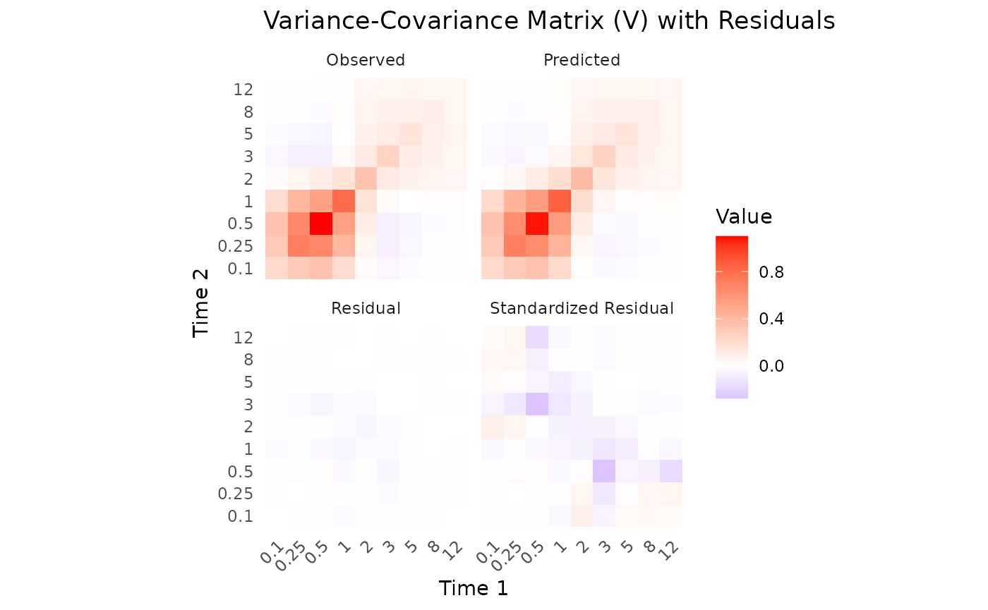
## $V
## 0.1 0.25 0.5 1 2 3
## 0.1 0.210318331 0.307810566 0.34863077 0.202610737 0.02244783 -0.04472722
## 0.25 0.307810566 0.707512991 0.65887098 0.416118052 0.05871261 -0.07441765
## 0.5 0.348630772 0.658870977 1.09983366 0.530554165 0.10572618 -0.07538386
## 1 0.202610737 0.416118052 0.53055416 0.803744604 0.16252833 0.02792441
## 2 0.022447834 0.058712608 0.10572618 0.162528331 0.34465070 0.12026872
## 3 -0.044727222 -0.074417647 -0.07538386 0.027924410 0.12026872 0.24989260
## 5 -0.018976800 -0.042420657 -0.04648286 0.001618855 0.07644080 0.11148574
## 8 -0.006630907 -0.011273701 -0.01981830 0.016197981 0.06398700 0.07493319
## 12 -0.005625994 -0.005018766 -0.01492001 0.014748325 0.04941463 0.05460018
## 5 8 12
## 0.1 -0.018976800 -0.006630907 -0.005625994
## 0.25 -0.042420657 -0.011273701 -0.005018766
## 0.5 -0.046482865 -0.019818299 -0.014920009
## 1 0.001618855 0.016197981 0.014748325
## 2 0.076440801 0.063987002 0.049414630
## 3 0.111485737 0.074933189 0.054600176
## 5 0.154215442 0.087680168 0.061332530
## 8 0.087680168 0.096530356 0.057621124
## 12 0.061332530 0.057621124 0.057988752
# Transform into mean and variance only format
examplomycin_aggregated_var <- examplomycin_aggregated
examplomycin_aggregated_var$V <- diag(diag(examplomycin_aggregated_var$V))

# View the structure of mean and variance only data
examplomycin_aggregated_var
## $E
## 0.1 0.25 0.5 1 2 3 5 8
## 0.966418 1.938774 2.787908 3.024706 2.257656 1.650808 1.063120 0.751180
## 12
## 0.512168
##
## $V
## [,1] [,2] [,3] [,4] [,5] [,6] [,7]
## [1,] 0.2103183 0.000000 0.000000 0.0000000 0.0000000 0.0000000 0.0000000
## [2,] 0.0000000 0.707513 0.000000 0.0000000 0.0000000 0.0000000 0.0000000
## [3,] 0.0000000 0.000000 1.099834 0.0000000 0.0000000 0.0000000 0.0000000
## [4,] 0.0000000 0.000000 0.000000 0.8037446 0.0000000 0.0000000 0.0000000
## [5,] 0.0000000 0.000000 0.000000 0.0000000 0.3446507 0.0000000 0.0000000
## [6,] 0.0000000 0.000000 0.000000 0.0000000 0.0000000 0.2498926 0.0000000
## [7,] 0.0000000 0.000000 0.000000 0.0000000 0.0000000 0.0000000 0.1542154
## [8,] 0.0000000 0.000000 0.000000 0.0000000 0.0000000 0.0000000 0.0000000
## [9,] 0.0000000 0.000000 0.000000 0.0000000 0.0000000 0.0000000 0.0000000
## [,8] [,9]
## [1,] 0.00000000 0.00000000
## [2,] 0.00000000 0.00000000
## [3,] 0.00000000 0.00000000
## [4,] 0.00000000 0.00000000
## [5,] 0.00000000 0.00000000
## [6,] 0.00000000 0.00000000
## [7,] 0.00000000 0.00000000
## [8,] 0.09653036 0.00000000
## [9,] 0.00000000 0.05798875Visualizing the Data
Before fitting the model, it’s helpful to visualize the data:
# Boxplot to visualize variability
ggplot(examplomycin, aes(x = TIME, y = DV, group = TIME)) +
  geom_boxplot(aes(group = TIME), width = 0.2) +
  labs(
    title = "Concentration Variability at Each Time Point",
    x = "Time (hours)",
    y = "Concentration (mg/L)"
  ) +
  theme_minimal()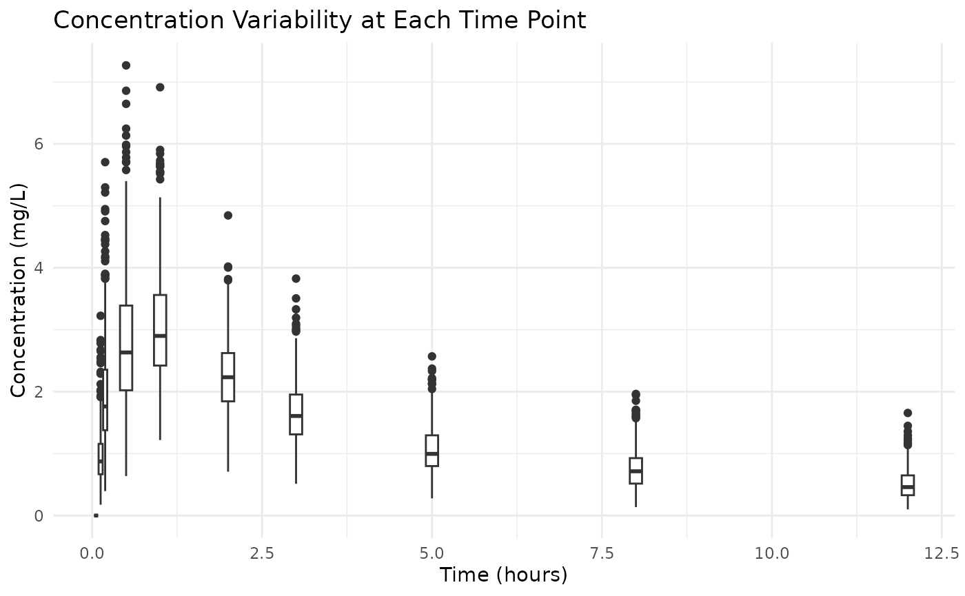
Model Specification
Defining the Pharmacokinetic Model
We’ll use a solved two-compartment model with first-order absorption:
Creating the Prediction Function
The prediction function is crucial for the admr package.
It: - Constructs the event table for dosing and sampling - Solves the
RxODE model - Returns predicted concentrations in the required
format
rxode2::rxSetSilentErr(1)## [1] TRUE
predder <- function(time, theta_i, dose = 100) {
    n_individuals <- nrow(theta_i)

    if (is.null(n_individuals)) {
      n_individuals <- 1
    }

    # Create event table
    ev <- eventTable(amount.units="mg", time.units="hours")
    ev$add.dosing(dose = dose, nbr.doses = 1, start.time = 0)
    ev$add.sampling(time)

    # Solve model
    out <- rxSolve(rxModel, params = theta_i, events = ev, cores = 0)

    # Format output
    cp_matrix <- matrix(out$cp, nrow = n_individuals, ncol = length(time),
                        byrow = TRUE)

    return(cp_matrix)
}
It can be observed that all steps for variance based modeling are similar to the mean and covariance based modeling. The only difference is in the data that is used for fitting the model.
Model Fitting
Setting Up Model Options
The genopts function creates an options object that
controls the model fitting process. We’ll do this twice: once for mean
and covariance data, and once for mean and variance only data.
Click here
opts_covar <- genopts(
  time = c(.1, .25, .5, 1, 2, 3, 5, 8, 12),  # Observation times
  p = list(
    beta = c(cl = 5, v1 = 10, v2 = 30, q = 10, ka = 1),  # Population parameters
    Omega = matrix(c(0.09, 0, 0, 0, 0,
                    0, 0.09, 0, 0, 0,
                    0, 0, 0.09, 0, 0,
                    0, 0, 0, 0.09, 0,
                    0, 0, 0, 0, 0.09), nrow = 5, ncol = 5),  # Random effects
    Sigma_prop = 0.04  # Proportional error
  ),
  nsim = 10000,  # Number of Monte Carlo samples
  n = 500,      # Number of individuals
  fo_appr = FALSE,  # Disable first-order approximation
  omega_expansion = 1,  # Omega expansion factor
  f = predder,    # Prediction function
  no_cov = FALSE # Use mean and covariance format
)


opts_var <- genopts(
  time = c(.1, .25, .5, 1, 2, 3, 5, 8, 12),  # Observation times
  p = list(
    beta = c(cl = 5, v1 = 10, v2 = 30, q = 10, ka = 1),  # Population parameters
    Omega = matrix(c(0.09, 0, 0, 0, 0,
                    0, 0.09, 0, 0, 0,
                    0, 0, 0.09, 0, 0,
                    0, 0, 0, 0.09, 0,
                    0, 0, 0, 0, 0.09), nrow = 5, ncol = 5),  # Random effects
    Sigma_prop = 0.04  # Proportional error
  ),
  nsim = 10000,  # Number of Monte Carlo samples
  n = 500,      # Number of individuals
  fo_appr = FALSE,  # Disable first-order approximation
  omega_expansion = 1,  # Omega expansion factor
  f = predder,    # Prediction function
  no_cov = TRUE # Use mean and variance only format
)
The only difference between the two options is the
no_cov argument, which is set to TRUE for
variance only data and FALSE for mean and covariance
data.
Fitting the Model
The fitIRMC function fits the model using the IRMC
algorithm:
fit.var <- admr::fitIRMC(
  opts = opts_var,
  obs = examplomycin_aggregated_var,
  chains = 6,  # Number of chains
  maxiter = 200,  # Maximum iterations
  use_grad = T
)
## Chain 1:
## Iter | NLL and Parameters (11 values)
## --------------------------------------------------------------------------------
## 1: -621.193 1.609 2.303 3.401 2.303 0.000 -2.408 -2.408 -2.408 -2.408 -2.408 -3.219
##
## ### Wide Search Phase ###
## 2: -630.798 1.593 2.057 3.463 2.177 -0.260 -2.086 -2.748 -2.349 -4.408 -1.915 -3.388
## 3: -633.204 1.598 2.055 3.456 2.172 -0.242 -2.126 -2.762 -2.352 -4.408 -1.967 -3.423
## 4: -633.204 1.598 2.055 3.456 2.173 -0.242 -2.126 -2.762 -2.352 -4.408 -1.967 -3.423
## Phase Wide Search Phase converged at iteration 4.
##
## ### Focussed Search Phase ###
## 5: -633.204 1.598 2.054 3.456 2.173 -0.242 -2.126 -2.762 -2.352 -4.408 -1.967 -3.423
## Phase Focussed Search Phase converged at iteration 5.
##
## ### Fine-Tuning Phase ###
## 6: -633.206 1.598 2.054 3.456 2.173 -0.243 -2.128 -2.761 -2.351 -4.408 -1.967 -3.418
## 7: -633.207 1.598 2.054 3.457 2.173 -0.243 -2.129 -2.761 -2.351 -4.408 -1.968 -3.418
## Phase Fine-Tuning Phase converged at iteration 7.
##
## ### Precision Phase ###
## 8: -633.207 1.597 2.054 3.457 2.173 -0.243 -2.129 -2.761 -2.351 -4.408 -1.968 -3.418
## Phase Precision Phase converged at iteration 8.
##
## Chain 1 Complete: Final NLL = -633.207, Time Elapsed = 8.74 seconds
##
## Phase Wide Search Phase converged at iteration 5.
## Phase Focussed Search Phase converged at iteration 6.
## Phase Fine-Tuning Phase converged at iteration 7.
## Phase Precision Phase converged at iteration 8.
##
## Chain 2 Complete: Final NLL = -633.201, Time Elapsed = 10.97 seconds
##
## Phase Wide Search Phase converged at iteration 5.
## Phase Focussed Search Phase converged at iteration 7.
## Phase Fine-Tuning Phase converged at iteration 8.
## Phase Precision Phase converged at iteration 9.
##
## Chain 3 Complete: Final NLL = -633.207, Time Elapsed = 16.18 seconds
##
## Phase Wide Search Phase converged at iteration 5.
## Phase Focussed Search Phase converged at iteration 6.
## Phase Fine-Tuning Phase converged at iteration 7.
## Phase Precision Phase converged at iteration 8.
##
## Chain 4 Complete: Final NLL = -633.207, Time Elapsed = 10.80 seconds
##
## Phase Wide Search Phase converged at iteration 5.
## Phase Focussed Search Phase converged at iteration 6.
## Phase Fine-Tuning Phase converged at iteration 7.
## Phase Precision Phase converged at iteration 8.
##
## Chain 5 Complete: Final NLL = -633.193, Time Elapsed = 11.81 seconds
##
## Phase Wide Search Phase converged at iteration 7.
## Phase Focussed Search Phase converged at iteration 9.
## Phase Fine-Tuning Phase converged at iteration 11.
## Phase Precision Phase converged at iteration 12.
##
## Chain 6 Complete: Final NLL = -633.211, Time Elapsed = 12.84 seconds
##
fit.covar <- admr::fitIRMC(
  opts = opts_covar,
  obs = examplomycin_aggregated,
  chains = 2,  # Number of chains
  maxiter = 200,  # Maximum iterations
  use_grad = T
)
## Chain 1:
## Iter | NLL and Parameters (11 values)
## --------------------------------------------------------------------------------
## 1: -1839.520 1.609 2.303 3.401 2.303 0.000 -2.408 -2.408 -2.408 -2.408 -2.408 -3.219
##
## ### Wide Search Phase ###
## 2: -1845.306 1.601 2.324 3.399 2.285 0.032 -2.274 -2.183 -2.325 -2.210 -2.418 -3.236
## 3: -1845.355 1.601 2.317 3.401 2.285 0.026 -2.283 -2.218 -2.338 -2.239 -2.387 -3.235
## 4: -1845.355 1.601 2.317 3.401 2.285 0.026 -2.283 -2.218 -2.338 -2.239 -2.387 -3.235
## 5: -1845.355 1.601 2.317 3.401 2.285 0.026 -2.283 -2.218 -2.338 -2.239 -2.387 -3.235
## 6: -1845.355 1.601 2.317 3.401 2.285 0.026 -2.282 -2.218 -2.338 -2.239 -2.387 -3.235
## 7: -1845.355 1.601 2.317 3.401 2.285 0.026 -2.282 -2.218 -2.338 -2.239 -2.387 -3.235
## Phase Wide Search Phase converged at iteration 7.
##
## ### Focussed Search Phase ###
## 8: -1845.355 1.601 2.317 3.401 2.285 0.026 -2.283 -2.218 -2.338 -2.239 -2.387 -3.235
## 9: -1845.355 1.601 2.317 3.401 2.285 0.026 -2.283 -2.218 -2.338 -2.239 -2.387 -3.235
## 10: -1845.355 1.601 2.317 3.401 2.285 0.026 -2.282 -2.218 -2.338 -2.239 -2.387 -3.235
## 11: -1845.355 1.601 2.317 3.401 2.285 0.026 -2.282 -2.218 -2.338 -2.239 -2.387 -3.235
## Phase Focussed Search Phase converged at iteration 11.
##
## ### Fine-Tuning Phase ###
## 12: -1845.355 1.601 2.317 3.401 2.285 0.026 -2.283 -2.218 -2.338 -2.239 -2.387 -3.235
## 13: -1845.355 1.601 2.317 3.401 2.285 0.026 -2.283 -2.218 -2.338 -2.239 -2.387 -3.235
## 14: -1845.355 1.601 2.317 3.401 2.285 0.026 -2.282 -2.218 -2.338 -2.239 -2.387 -3.235
## 15: -1845.355 1.601 2.317 3.401 2.285 0.026 -2.282 -2.218 -2.338 -2.239 -2.387 -3.235
## Phase Fine-Tuning Phase converged at iteration 15.
##
## ### Precision Phase ###
## 16: -1845.355 1.601 2.317 3.401 2.285 0.026 -2.283 -2.218 -2.338 -2.239 -2.387 -3.235
## 17: -1845.355 1.601 2.317 3.401 2.285 0.026 -2.283 -2.218 -2.338 -2.239 -2.387 -3.235
## 18: -1845.355 1.601 2.317 3.401 2.285 0.026 -2.282 -2.218 -2.338 -2.239 -2.387 -3.235
## 19: -1845.355 1.601 2.317 3.401 2.285 0.026 -2.282 -2.218 -2.338 -2.239 -2.387 -3.235
## Phase Precision Phase converged at iteration 19.
##
## Chain 1 Complete: Final NLL = -1845.355, Time Elapsed = 13.84 seconds
##
## Phase Focussed Search Phase converged at iteration 50.
## Phase Fine-Tuning Phase converged at iteration 51.
## Phase Precision Phase converged at iteration 52.
##
## Chain 2 Complete: Final NLL = -1845.354, Time Elapsed = 41.86 seconds
## Convergence speeds up a lot for the variance fit when using gradients, as the optimization landscape is more challenging with less information. However NLL is slightly worse than without gradients. This is likely due to local minima issues, which can be alleviated by using more chains, larger MC samples, or more iterations.
Model Diagnostics
Basic Diagnostics
The print method provides a summary of the model
fit:
print(fit.var)## -- FitIRMC Summary --
##
## -- Objective Function and Information Criteria --
## Log-likelihood: -633.2115
## AIC: 1277.42
## BIC: 1334.78
## Condition#(Cov): 503.86
## Condition#(Cor): 721.40
##
## -- Timing Information --
## Best Chain: 12.8447 seconds
## All Chains: 71.3397 seconds
## Covariance: 23.9114 seconds
## Elapsed: 95.25 seconds
##
## -- Population Parameters --
## # A tibble: 6 × 6
## Parameter Est. SE `%RSE` `Back-transformed(95%CI)` `BSV(CV%)`
## <chr> <dbl> <dbl> <dbl> <chr> <dbl>
## 1 cl 1.60 0.0220 1.37 4.95 (4.74, 5.17) 34.3
## 2 v1 2.08 0.114 5.48 8.02 (6.41, 10.02) 26.7
## 3 v2 3.45 0.0555 1.61 31.49 (28.25, 35.11) 30.6
## 4 q 2.19 0.0385 1.76 8.90 (8.25, 9.59) 12.5
## 5 ka -0.216 0.106 49.1 0.81 (0.65, 0.99) 36.4
## 6 Residual Error 0.0339 NA NA 0.0339 NA
##
## -- Iteration Diagnostics --
## Iter | NLL and Parameters
## --------------------------------------------------------------------------------
## 1: -438.962 1.470 2.437 3.397 2.216 0.000 -2.331 -2.526 -1.768 -2.003 -2.220 -2.989
## 2: -632.547 1.599 2.481 3.362 2.255 0.166 -2.204 -2.371 -1.996 -2.152 -2.060 -3.538
## 3: -632.074 1.594 2.080 3.445 2.186 -0.230 -2.124 -2.625 -2.403 -4.152 -2.010 -3.411
## 4: -633.173 1.600 2.076 3.448 2.181 -0.223 -2.125 -2.626 -2.403 -4.152 -2.010 -3.411
## 5: -633.182 1.600 2.076 3.448 2.180 -0.223 -2.125 -2.626 -2.402 -4.152 -2.011 -3.410
## ... (omitted iterations) ...
## 8: -633.211 1.599 2.082 3.450 2.186 -0.216 -2.141 -2.642 -2.371 -4.155 -2.021 -3.383
## 9: -633.211 1.599 2.082 3.450 2.186 -0.216 -2.141 -2.642 -2.371 -4.155 -2.021 -3.383
## 10: -633.211 1.599 2.082 3.450 2.185 -0.216 -2.140 -2.642 -2.371 -4.155 -2.021 -3.383
## 11: -633.211 1.599 2.081 3.450 2.186 -0.216 -2.140 -2.642 -2.371 -4.155 -2.021 -3.383
## 12: -633.211 1.599 2.081 3.450 2.186 -0.216 -2.140 -2.642 -2.370 -4.155 -2.021 -3.383
print(fit.covar)## -- FitIRMC Summary --
##
## -- Objective Function and Information Criteria --
## Log-likelihood: -1845.3554
## AIC: 3701.71
## BIC: 3759.07
## Condition#(Cov): 152.17
## Condition#(Cor): 216.85
##
## -- Timing Information --
## Best Chain: 13.8393 seconds
## All Chains: 55.6998 seconds
## Covariance: 23.3068 seconds
## Elapsed: 79.01 seconds
##
## -- Population Parameters --
## # A tibble: 6 × 6
## Parameter Est. SE `%RSE` `Back-transformed(95%CI)` `BSV(CV%)`
## <chr> <dbl> <dbl> <dbl> <chr> <dbl>
## 1 cl 1.60 0.0152 0.950 4.96 (4.81, 5.11) 31.9
## 2 v1 2.32 0.0865 3.73 10.14 (8.56, 12.02) 33.0
## 3 v2 3.40 0.0400 1.18 30.00 (27.74, 32.45) 31.1
## 4 q 2.29 0.0212 0.928 9.83 (9.43, 10.24) 32.6
## 5 ka 0.0263 0.0817 311. 1.03 (0.87, 1.20) 30.3
## 6 Residual Error 0.0394 NA NA 0.0394 NA
##
## -- Iteration Diagnostics --
## Iter | NLL and Parameters
## --------------------------------------------------------------------------------
## 1: -1839.520 1.609 2.303 3.401 2.303 0.000 -2.408 -2.408 -2.408 -2.408 -2.408 -3.219
## 2: -1845.306 1.601 2.324 3.399 2.285 0.032 -2.274 -2.183 -2.325 -2.210 -2.418 -3.236
## 3: -1845.355 1.601 2.317 3.401 2.285 0.026 -2.283 -2.218 -2.338 -2.239 -2.387 -3.235
## 4: -1845.355 1.601 2.317 3.401 2.285 0.026 -2.283 -2.218 -2.338 -2.239 -2.387 -3.235
## 5: -1845.355 1.601 2.317 3.401 2.285 0.026 -2.283 -2.218 -2.338 -2.239 -2.387 -3.235
## ... (omitted iterations) ...
## 15: -1845.355 1.601 2.317 3.401 2.285 0.026 -2.282 -2.218 -2.338 -2.239 -2.387 -3.235
## 16: -1845.355 1.601 2.317 3.401 2.285 0.026 -2.283 -2.218 -2.338 -2.239 -2.387 -3.235
## 17: -1845.355 1.601 2.317 3.401 2.285 0.026 -2.283 -2.218 -2.338 -2.239 -2.387 -3.235
## 18: -1845.355 1.601 2.317 3.401 2.285 0.026 -2.282 -2.218 -2.338 -2.239 -2.387 -3.235
## 19: -1845.355 1.601 2.317 3.401 2.285 0.026 -2.282 -2.218 -2.338 -2.239 -2.387 -3.235Convergence Assessment
The plot method visualizes the convergence of the model
fit:
plot(fit.var)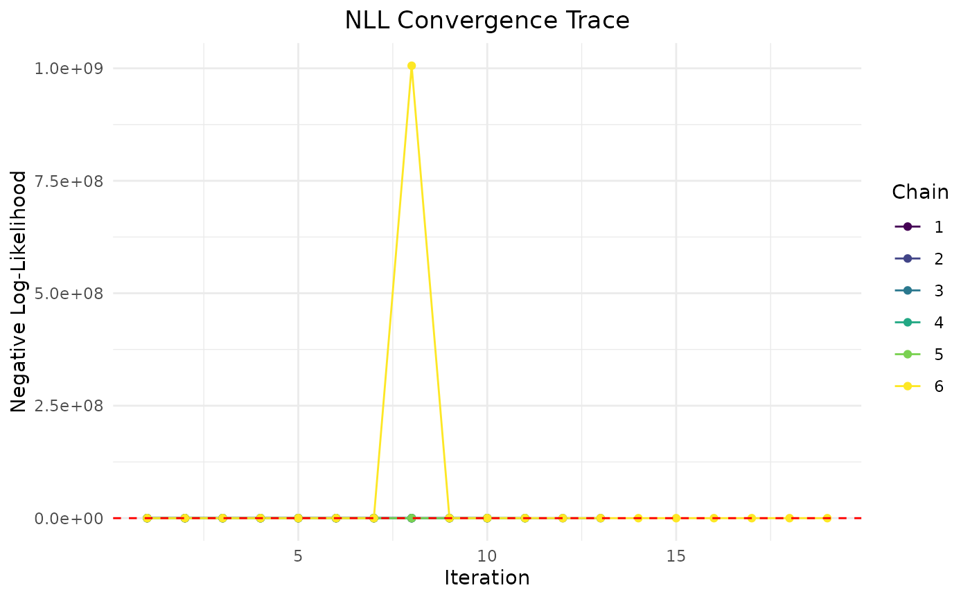
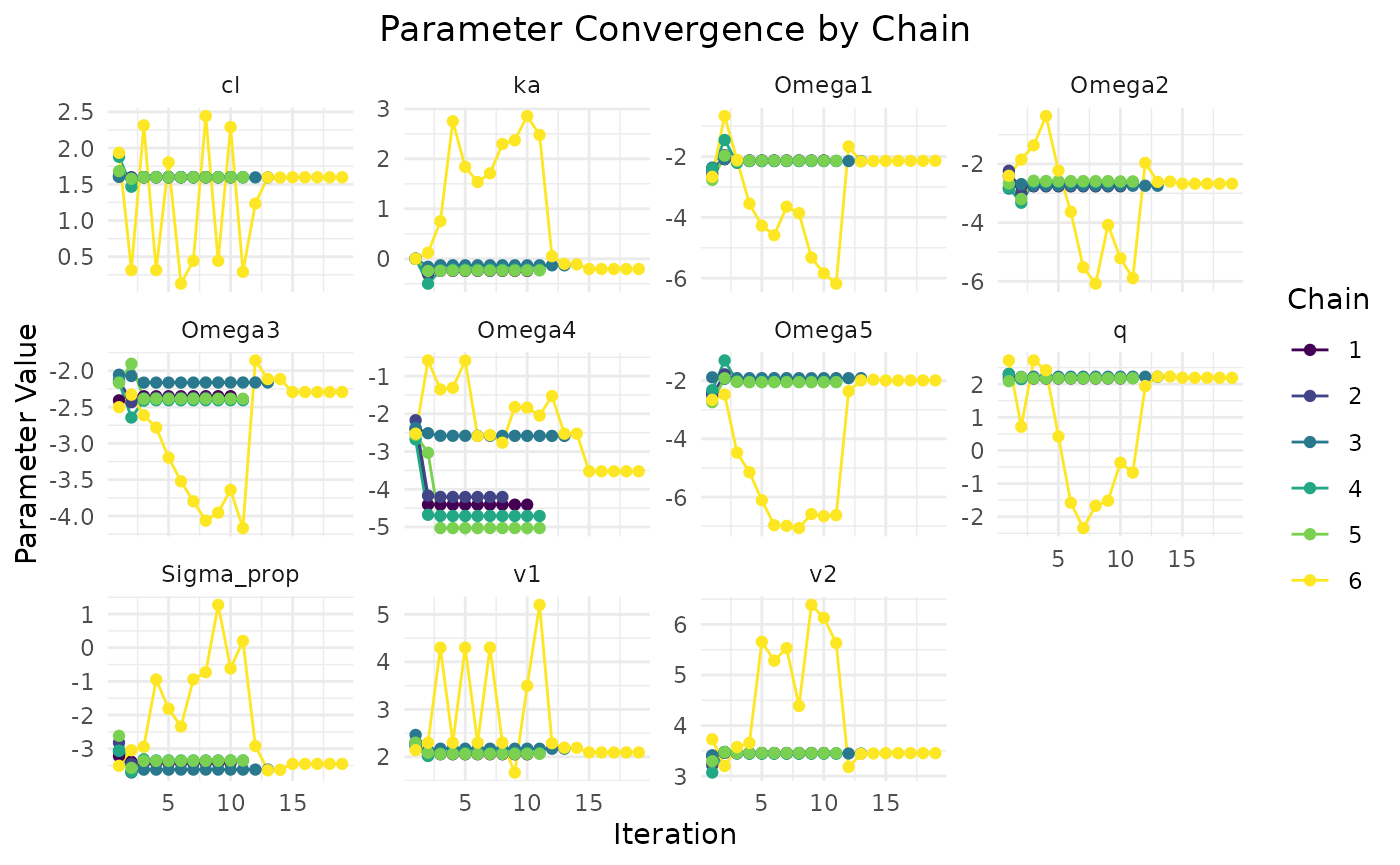
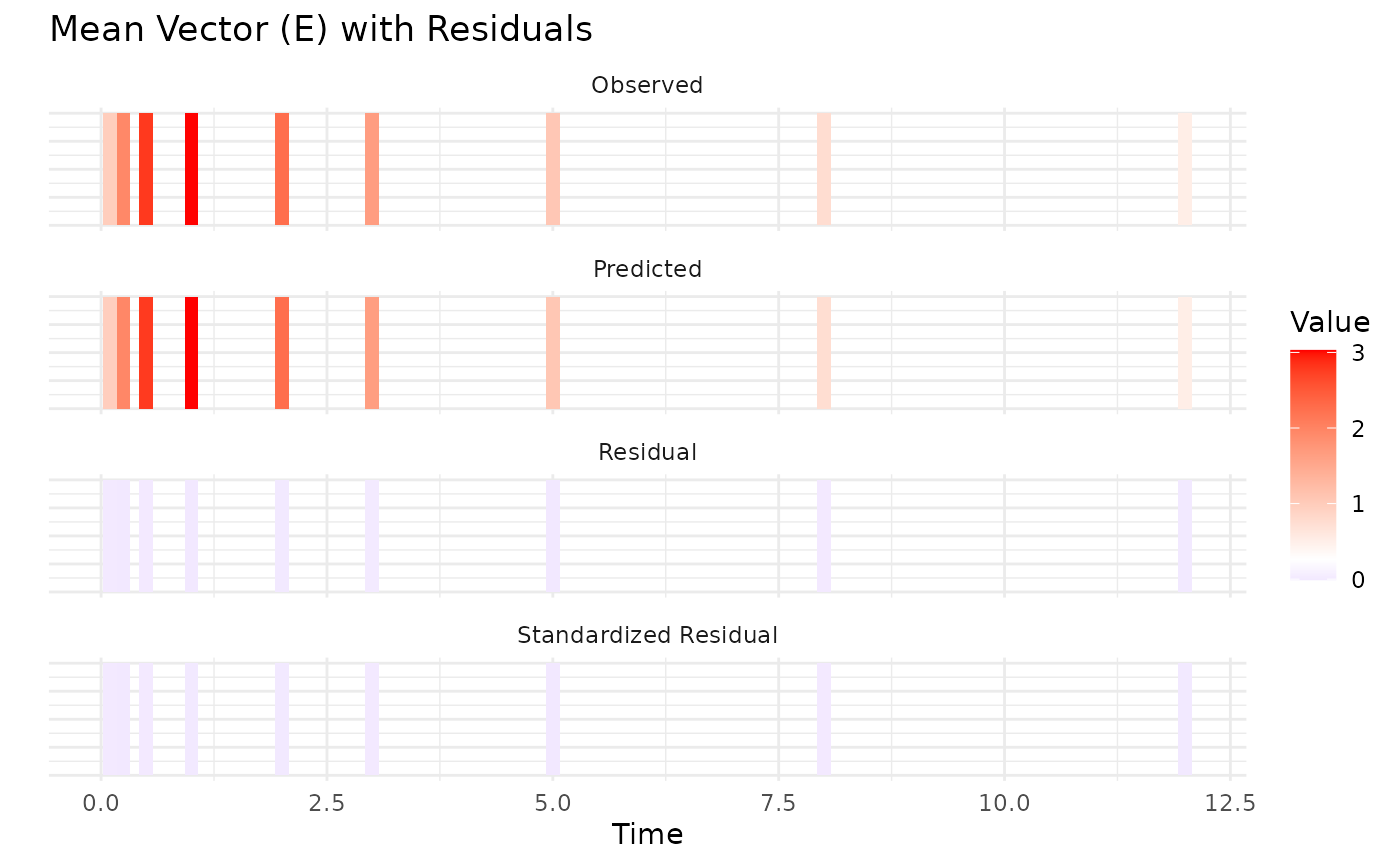
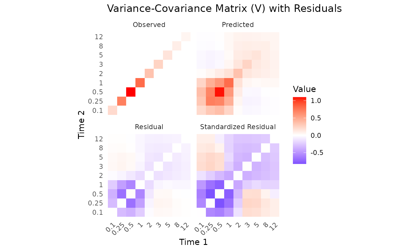 First variance only data is plotted. We see that the model converges
reasonbly well within the specified iterations, with some parameters
showing more variability across chains.
First variance only data is plotted. We see that the model converges
reasonbly well within the specified iterations, with some parameters
showing more variability across chains.
Now we plot the mean and covariance data fit:
plot(fit.covar)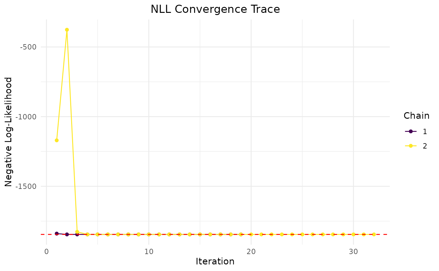
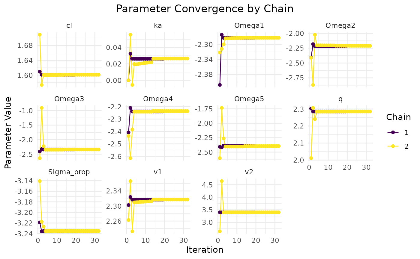


 This data seems to converge slightly better, especially when looking at
chain comparisons. All chains converge to similar values, whereas in the
variance only data, the chains show more variability while resulting in
the same NLL. This is due to non-identifiability issues of some
parameters when only variance data is used.
This data seems to converge slightly better, especially when looking at
chain comparisons. All chains converge to similar values, whereas in the
variance only data, the chains show more variability while resulting in
the same NLL. This is due to non-identifiability issues of some
parameters when only variance data is used.
True vs Estimated Parameters
Given that true parameter estimates are known, we can compare the estimated parameters to the true values:
params.true <- list(
  beta = c(cl = 5, v1 = 10, v2 = 30, q = 10, ka = 1),
  Omega = diag(rep(0.09, 5)),
  Sigma_prop = 0.04
)
cat("True parameter values:\n")
## True parameter values:
print(params.true)## $beta
## cl v1 v2 q ka
## 5 10 30 10 1
##
## $Omega
## [,1] [,2] [,3] [,4] [,5]
## [1,] 0.09 0.00 0.00 0.00 0.00
## [2,] 0.00 0.09 0.00 0.00 0.00
## [3,] 0.00 0.00 0.09 0.00 0.00
## [4,] 0.00 0.00 0.00 0.09 0.00
## [5,] 0.00 0.00 0.00 0.00 0.09
##
## $Sigma_prop
## [1] 0.04
cat("Estimated parameters (mean and variance only):\n")## Estimated parameters (mean and variance only):
print(fit.var$transformed_params)## $beta
## cl v1 v2 q ka
## 4.9478613 8.0163852 31.4926556 8.8953771 0.8058678
##
## $Omega
## [,1] [,2] [,3] [,4] [,5]
## [1,] 0.1175999 0.00000000 0.00000000 0.00000000 0.0000000
## [2,] 0.0000000 0.07120286 0.00000000 0.00000000 0.0000000
## [3,] 0.0000000 0.00000000 0.09343625 0.00000000 0.0000000
## [4,] 0.0000000 0.00000000 0.00000000 0.01568346 0.0000000
## [5,] 0.0000000 0.00000000 0.00000000 0.00000000 0.1325419
##
## $Sigma_prop
## [1] 0.03394168We observe that both methods recover the true parameters reasonably well, but the mean and covariance method provides more accurate estimates due to the additional information from covariances. In this example model, especially inter-compartmental clearance (q) and its random effect are more challenging to estimate accurately with only variance data. However, using larger sample sizes from more studies will help improve the estimates from both data. To further illustrate the differences in dynamics, we can simulate concentration-time profiles using the true parameters and the estimated parameters from both methods.
Dosing plot with Confidence Intervals for true vs estimated parameters
Let’s simulate concentration-time profiles using the true parameters and the estimated parameters from both methods, and then plot the results with confidence intervals. First, we define the models using the true parameters and the estimated parameters from both methods:
Click here
params.true <- list(
  beta = c(cl = 5, v1 = 10, v2 = 30, q = 10, ka = 1),
  Omega = diag(rep(0.09, 5)),
  Sigma_prop = 0.04
)

params.covar <- fit.covar$transformed_params
params.var <- fit.var$transformed_params

rxModel_true <- function(){
  ini({
    cl <- params.true$beta["cl"]  # Clearance
    v1 <- params.true$beta["v1"]  # Volume of central compartment
    v2 <- params.true$beta["v2"] # Volume of peripheral compartment
    q <- params.true$beta["q"]    # Inter-compartmental clearance
    ka <- params.true$beta["ka"]   # Absorption rate constant

    eta_cl ~ params.true$Omega[1,1]
    eta_v1 ~ params.true$Omega[2,2]
    eta_v2 ~ params.true$Omega[3,3]
    eta_q ~ params.true$Omega[4,4]
    eta_ka ~ params.true$Omega[5,5]
  })
  model({
    cl <- cl * exp(eta_cl)
    v1 <- v1 * exp(eta_v1)
    v2 <- v2 * exp(eta_v2)
    q <- q * exp(eta_q)
    ka <- ka * exp(eta_ka)
    cp = linCmt(cl, v1, v2, q, ka)
  })
}
rxModel_covar <- function(){
  ini({
    cl <- params.covar$beta["cl"]  # Clearance
    v1 <- params.covar$beta["v1"]  # Volume of central compartment
    v2 <- params.covar$beta["v2"] # Volume of peripheral compartment
    q <- params.covar$beta["q"]    # Inter-compartmental clearance
    ka <- params.covar$beta["ka"]   # Absorption rate constant

    eta_cl ~ params.covar$Omega[1,1]
    eta_v1 ~ params.covar$Omega[2,2]
    eta_v2 ~ params.covar$Omega[3,3]
    eta_q ~ params.covar$Omega[4,4]
    eta_ka ~ params.covar$Omega[5,5]
  })
  model({
    cl <- cl * exp(eta_cl)
    v1 <- v1 * exp(eta_v1)
    v2 <- v2 * exp(eta_v2)
    q <- q * exp(eta_q)
    ka <- ka * exp(eta_ka)
    cp = linCmt(cl, v1, v2, q, ka)
  })
}
rxModel_var <- function(){
  ini({
    cl <- params.var$beta["cl"]  # Clearance
    v1 <- params.var$beta["v1"]  # Volume of central compartment
    v2 <- params.var$beta["v2"] # Volume of peripheral compartment
    q <- params.var$beta["q"]    # Inter-compartmental clearance
    ka <- params.var$beta["ka"]   # Absorption rate constant

    eta_cl ~ params.var$Omega[1,1]
    eta_v1 ~ params.var$Omega[2,2]
    eta_v2 ~ params.var$Omega[3,3]
    eta_q ~ params.var$Omega[4,4]
    eta_ka ~ params.var$Omega[5,5]
  })
  model({
    cl <- cl * exp(eta_cl)
    v1 <- v1 * exp(eta_v1)
    v2 <- v2 * exp(eta_v2)
    q <- q * exp(eta_q)
    ka <- ka * exp(eta_ka)
    cp = linCmt(cl, v1, v2, q, ka)
  })
}

rxModel_true <- rxode2(rxModel_true())
rxModel_true <- rxModel_true$simulationModel
rxModel_covar <- rxode2(rxModel_covar())
rxModel_covar <- rxModel_covar$simulationModel
rxModel_var <- rxode2(rxModel_var())
rxModel_var <- rxModel_var$simulationModel
Now we can simulate the concentration-time profiles and plot the results:
time_points <- seq(0, 12, by = 0.01)  # Dense time points for smooth curves
ev <- eventTable(amount.units="mg", time.units="hours")
ev$add.dosing(dose = 100, nbr.doses = 2, dosing.interval = 6)
ev$add.sampling(time_points)


sim_true <- rxSolve(rxModel_true, events = ev, cores = 0, nSub = 10000)
sim_covar <- rxSolve(rxModel_covar, events = ev, cores = 0, nSub = 10000)
sim_var <- rxSolve(rxModel_var, events = ev, cores = 0, nSub = 10000)

# Combine the confidence intervals with a label for the model
ci_true <- as.data.frame(confint(sim_true, "cp", level=0.95)) %>%
  mutate(Model = "True parameters")
## summarizing data...done
ci_covar <- as.data.frame(confint(sim_covar, "cp", level=0.95)) %>%
  mutate(Model = "Covariance fit")
## summarizing data...done
ci_var <- as.data.frame(confint(sim_var, "cp", level=0.95)) %>%
  mutate(Model = "Variance fit")
## summarizing data...done
# Bind them together
ci_true_covar <- bind_rows(ci_true, ci_covar) %>%
  mutate(
    p1 = as.numeric(as.character(p1)),
    Percentile = factor(Percentile, levels = unique(Percentile[order(p1)]))
  )

ci_true_var <- bind_rows(ci_true, ci_var) %>%
  mutate(
    p1 = as.numeric(as.character(p1)),
    Percentile = factor(Percentile, levels = unique(Percentile[order(p1)]))
  )


# Plot both models
ggplot(ci_true_covar, aes(x = time, group = interaction(Model, Percentile))) +
  geom_ribbon(aes(ymin = p2.5, ymax = p97.5, fill = Model),
              alpha = 0.2, colour = NA) +
  geom_line(aes(y = p50, colour = Model), size = 0.8) +
  labs(
    title = "Central Concentration Simulations",
    x = "Time",
    y = "Central Concentration (mg/L)"
  ) +
  theme_bw(base_size = 14) +
  scale_colour_manual(values = c("True parameters" = "blue",
                                 "Covariance fit" = "red")) +
  scale_fill_manual(values = c("True parameters" = "blue",
                               "Covariance fit" = "red")) +
  coord_cartesian(xlim = c(0, 12), ylim = c(0, 7))
## Warning: Using `size` aesthetic for lines was deprecated in ggplot2 3.4.0.
## ℹ Please use `linewidth` instead.
## This warning is displayed once per session.
## Call `lifecycle::last_lifecycle_warnings()` to see where this warning was
## generated.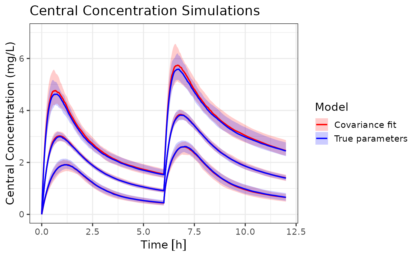
ggplot(ci_true_var, aes(x = time, group = interaction(Model, Percentile))) +
geom_ribbon(aes(ymin = p2.5, ymax = p97.5, fill = Model),
alpha = 0.2, colour = NA) +
geom_line(aes(y = p50, colour = Model), size = 0.8) +
labs(
title = "Central Concentration Simulations",
x = "Time",
y = "Central Concentration (mg/L)"
) +
theme_bw(base_size = 14) +
scale_colour_manual(values = c("True parameters" = "blue",
"Variance fit" = "darkgreen")) +
scale_fill_manual(values = c("True parameters" = "blue",
"Variance fit" = "darkgreen")) +
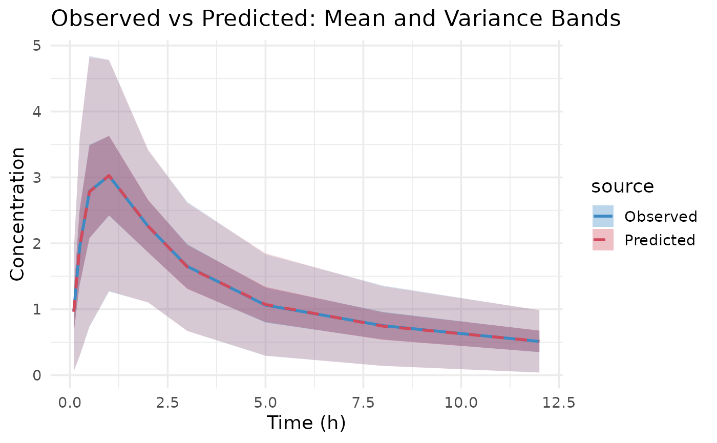
coord_cartesian(xlim = c(0, 12), ylim = c(0, 7))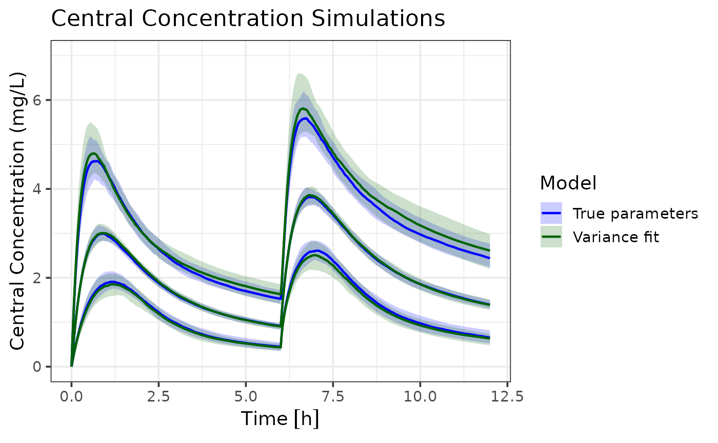 Both models capture the central tendency of the true parameters dynamics
well. However, the variance only model shows slightly wider population
intervals. In this scenario this isn’t very problematic, since a wider
range still captures the true dynamics. However, in other scenarios,
this could lead to over- or under-prediction of certain percentiles. The
estimation error is expected due to the reduced information content in
variance-only data.
Both models capture the central tendency of the true parameters dynamics
well. However, the variance only model shows slightly wider population
intervals. In this scenario this isn’t very problematic, since a wider
range still captures the true dynamics. However, in other scenarios,
this could lead to over- or under-prediction of certain percentiles. The
estimation error is expected due to the reduced information content in
variance-only data.
Best Practices
So to recap, here are some best practices for variance-based (but
also covariance-based) modeling with admr:
-
Data Preparation:
- Always check your data for missing values and outliers
- Ensure time points are consistent across subjects
- Consider the impact of dosing events on your analysis
-
Model Specification:
- Start with a simple model and gradually add complexity
- Use meaningful initial values for parameters
- Consider parameter transformations for better estimation
-
Model Fitting:
- Use multiple chains to improve optimization
- Monitor convergence carefully
- Check parameter estimates for biological plausibility
-
Diagnostics:
- Always examine convergence plots
- Validate model predictions against observed data
For more information, see the package documentation and other vignettes.