Creating the Examplomycin Dataset
This vignette demonstrates how to create a simulated pharmacokinetic
dataset for a fictional drug called examplomycin. The dataset is
designed to showcase the capabilities of the admr package
for aggregate data modeling.
Overview
The examplomycin dataset is a simulated pharmacokinetic study with the following characteristics: - 500 healthy subjects - Single oral dose of 100 mg - 9 sampling time points per subject - Two-compartment model with first-order absorption - Random effects on all parameters - Proportional residual error
Data Generation Function
The generate_data function creates the examplomycin
dataset with the following features:
Two-compartment model with first-order absorption
Log-normal random effects on all parameters
Proportional residual error
Standardized sampling schedule
nlmixr2-compatible data format
Show code
generate_data <- function(n, times, seed = 1) {
  set.seed(seed)

  # Define the pharmacokinetic model
  mod <- function(){
    model({
    # Parameters
    ke = cl / v1             # Elimination rate constant
    k12 = q / v1             # Rate constant for central to peripheral transfer
    k21 = q / v2             # Rate constant for peripheral to central transfer

    # Differential equations for drug amount in compartments
    d/dt(depot)    = -ka * depot
    d/dt(central)  = ka * depot - ke * central -
      k12 * central +
      k21 * peripheral
    d/dt(peripheral) = k12 * central -
      k21 * peripheral

    # Concentration in the central compartment
    cp = central / v1
    })

  }

  mod <- rxode2(mod)
  mod <- mod$simulationModel

  # Population parameters
  theta <- c(cl = 5, v1 = 10, v2 = 30, q = 10, ka = 1)

  # Correlation matrix for random effects
  omegaCor <- matrix(c(1,  0,  0,  0,  0,
                       0,  1,  0,  0,  0,
                       0,  0,  1,  0,  0,
                       0,  0,  0,  1,  0,
                       0,  0,  0,  0,  1),
                     dimnames = list(NULL, c("eta.cl", "eta.v1", "eta.v2", "eta.q",
                                           "eta.ka")), nrow = 5)

  # Standard deviations of random effects
  iiv.sd <- c(0.3, 0.3, 0.3, 0.3, 0.3)

  # Create covariance matrix
  iiv <- iiv.sd %*% t(iiv.sd)
  omega <- iiv * omegaCor

  # Generate random effects
  mv <- mvrnorm(n, rep(0, dim(omega)[1]), omega)

  # Create individual parameters
  params.all <-
    data.table(
      "ID" = seq(1:n),
      "cl" = theta['cl'] * exp(mv[, 1]),
      "v1" = theta['v1'] * exp(mv[, 2]),
      "v2" = theta['v2'] * exp(mv[, 3]),
      "q"  = theta['q']  * exp(mv[, 4]),
      "ka" = theta['ka'] * exp(mv[, 5])
    )

  # Create event table
  ev <- et() %>%
    et(amt = 100) %>%  # Single dose
    et(0) %>%  # Initial time point
    et(times) %>%  # Sampling schedule
    et(ID = seq(1, n)) %>%  # Subject IDs
    as.data.frame()

  # Solve the model
  sim <- rxSolve(mod, events = ev, iCov = params.all, cores = 0, addCov = T) %>%
    mutate(ID = as.integer(id), TIME = as.numeric(time)) %>%
    dplyr::select(-c(id, time)) %>%
    mutate(AMT = ifelse(TIME == 0, 100, 0)) %>%
    mutate(EVID = ifelse(TIME == 0, 101, 0)) %>%
    mutate(CMT = ifelse(TIME == 0, 1, 2))

  # Add residual error
  sim$rv <- rnorm(nrow(sim), 0, 0.2)
  sim$DV <- round(sim$cp * (1 + sim$rv), 3)
  sim <- merge(sim, params.all)

  # Select final columns
  dat <- sim %>%
    dplyr::select("ID", "TIME", "DV", "AMT", "EVID", "CMT")

  return(dat)
}
Generating the Dataset
We’ll generate the examplomycin dataset with: - 500 subjects - 9 time points (0.1, 0.25, 0.5, 1, 2, 3, 5, 8, 12 hours) - Random seed for reproducibility
examplomycin <- generate_data(
  n = 500,  # Number of subjects
  times = c(.1, .25, .5, 1, 2, 3, 5, 8, 12),  # Sampling times
  seed = 1  # Random seed
)
## ℹ parameter labels from comments are typically ignored in non-interactive mode## ℹ Need to run with the source intact to parse comments
head(examplomycin)## ID TIME DV AMT EVID CMT
## 1 460 0.00 0.000 100 101 1
## 2 460 0.10 0.752 0 0 2
## 3 460 0.25 1.932 0 0 2
## 4 460 0.50 3.694 0 0 2
## 5 460 1.00 3.479 0 0 2
## 6 460 2.00 4.003 0 0 2Saving the Dataset
The dataset is saved as a package data object for use in other vignettes and examples:
Visualizing the Dataset
We’ll create a concentration-time plot to visualize the simulated data:
# Create concentration-time plot
ggplot(examplomycin, aes(x = TIME, y = DV, color = factor(ID))) +
  geom_line(alpha = 0.7) +    # Connect points with lines
  geom_point(size = 2, alpha = 0.8) +  # Add observation points
  scale_color_viridis_d(name = "Subject ID") +  # Color by subject
  labs(
    title = "Concentration-Time Profile",
    x = "Time (hours)",
    y = "Observed Concentration (DV)"
  ) +
  theme_minimal() +
  theme(legend.position = "none")  # Hide legend for clarity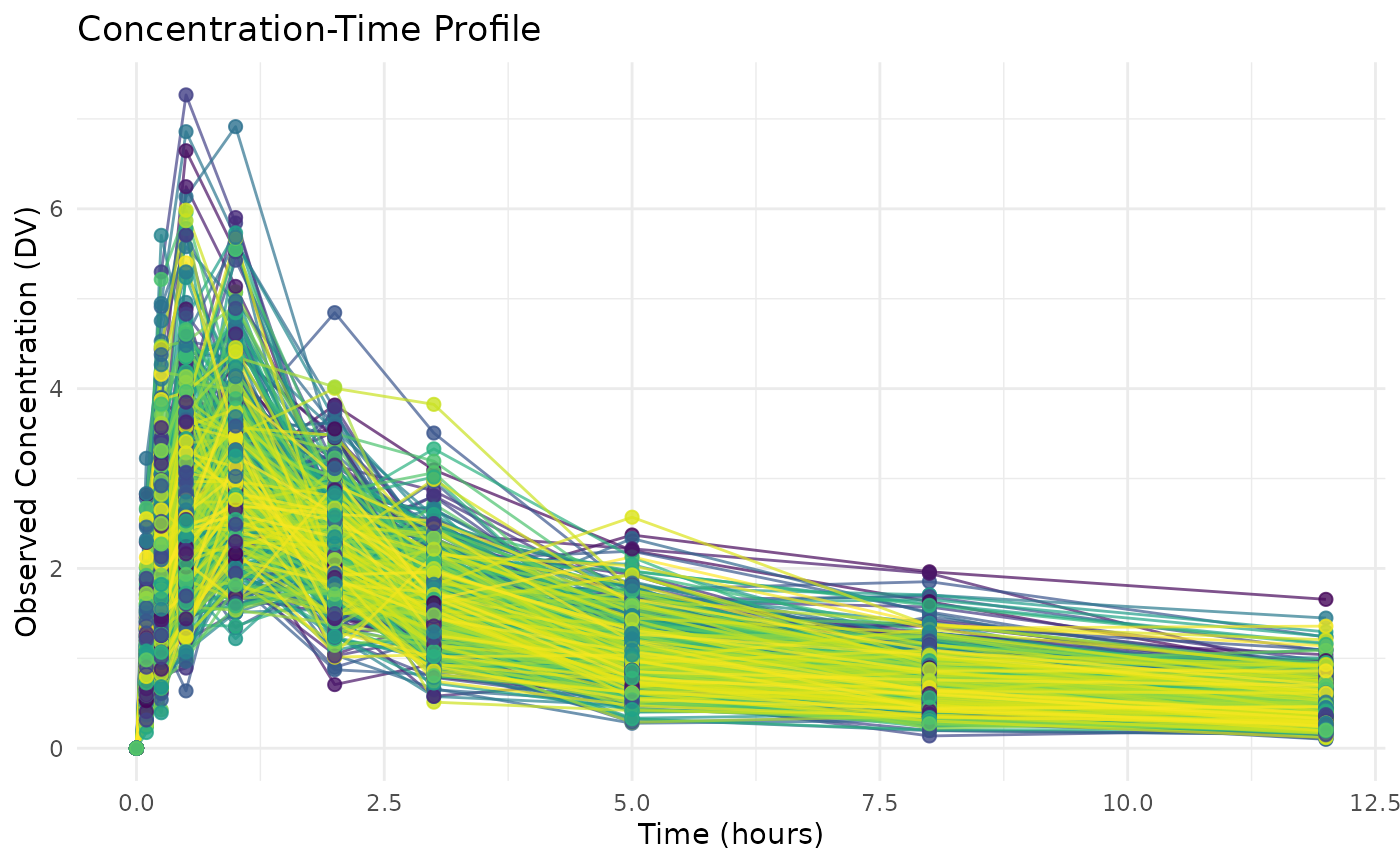
Dataset Structure
The examplomycin dataset contains the following columns:
ID: Subject identifierTIME: Observation time (hours)DV: Observed concentrationAMT: Dose amount (100 mg or NA)EVID: Event type (101 for dose, 0 for observation)CMT: Compartment number (1 for depot, 2 for central)
This dataset serves as a realistic example for demonstrating
aggregate data modeling techniques in the admr package.