Introduction to Aggregate Data Modeling with admr
This vignette provides an introduction to using multiple datasets
with the admr package in R. This is an example how to
combine different datasets with non-overlapping timepoints. However, the
same principles can be applied to datasets with overlapping timepoints;
or even datasets with different dosing regimens. Therefore, this
vignette can be used as a guide for meta-analysis of pharmacokinetic
data. Further research is currently being conducted to validate this
approach for meta-analysis or model averaging.
Understanding the Data Format
The admr package works with two types of data
formats:
- Raw Data: Individual-level observations in a wide or long format.
- Aggregate Data: Summary statistics (mean and covariance) computed from raw data.
- Aggregate Data with only means and variance: Mean and variance for each time point (no covariances).
The vignette Variance-only based modelling provides more details on the third option.
Let’s look at the simulated examplomycin dataset, which we’ll use throughout this vignette:
##    ID TIME    DV AMT EVID CMT
## 1 460 0.00 0.000 100  101   1
## 2 460 0.10 0.752   0    0   2
## 3 460 0.25 1.932   0    0   2
## 4 460 0.50 3.694   0    0   2
## 5 460 1.00 3.479   0    0   2
## 6 460 2.00 4.003 0 0 2## Number of subjects: 500## Number of time points: 10## Time points: 0, 0.1, 0.25, 0.5, 1, 2, 3, 5, 8, 12Data Preparation
Converting Raw Data to Aggregate Format
The first step is to convert our simulated raw data into aggregate
format. In real-world scenarios, you might have to extract summary
statistics from published studies, depending on the available
information. But for this example, we’ll compute the mean and covariance
from the examplomycin dataset. Here’s how to do it:
# Convert to wide format
examplomycin_wide <- examplomycin %>%
  filter(EVID != 101) %>%  # Remove dosing events
  dplyr::select(ID, TIME, DV) %>%  # Select relevant columns
  pivot_wider(names_from = TIME, values_from = DV) %>%  # Convert to wide format
  dplyr::select(-c(1))  # Remove ID column
To illustrate the use of multiple datasets, we’ll split the data into two groups based on timepoints: one group with timepoints 0.1, 0.25, 0.5, and 1 hour; and another group with timepoints 2, 3, 5, 8, and 12 hours. This illustrates how to use a dataset with absorption phase data and a dataset with elimination phase data. We will then create aggregated data for each group separately:
# Create aggregated data and filter timepoints 1 to 4
examplomycin_aggregated1 <- examplomycin_wide %>%
  dplyr::select(c(1:4)) %>%
  meancov()

examplomycin_aggregated2 <- examplomycin_wide %>%
  dplyr::select(c(5:9)) %>%
  meancov()

# View the structure of aggregated data
str(examplomycin_aggregated1)
## List of 2
## $ E: Named num [1:4] 0.966 1.939 2.788 3.025
## ..- attr(*, "names")= chr [1:4] "0.1" "0.25" "0.5" "1"
## $ V: num [1:4, 1:4] 0.21 0.308 0.349 0.203 0.308 ...
## ..- attr(*, "dimnames")=List of 2
## .. ..$ : chr [1:4] "0.1" "0.25" "0.5" "1"
## .. ..$ : chr [1:4] "0.1" "0.25" "0.5" "1"
str(examplomycin_aggregated2)## List of 2
## $ E: Named num [1:5] 2.258 1.651 1.063 0.751 0.512
## ..- attr(*, "names")= chr [1:5] "2" "3" "5" "8" ...
## $ V: num [1:5, 1:5] 0.3447 0.1203 0.0764 0.064 0.0494 ...
## ..- attr(*, "dimnames")=List of 2
## .. ..$ : chr [1:5] "2" "3" "5" "8" ...
## .. ..$ : chr [1:5] "2" "3" "5" "8" ...Compared to the full aggregated dataset, each of these datasets
contains only a subset of the timepoints. This means covariances between
timepoints in different datasets are not available, effectively reducing
the information content. However, the admr package can
still handle this situation effectively.
Visualizing the Data
Before fitting the model, it’s helpful to visualize the data:
# Give different colours to 1-4 and 5-9
examplomycin <- admr::examplomycin %>%
  filter(EVID != 101) %>%  # Remove dosing events
  mutate(TIME = factor(TIME, levels = c(0.1, 0.25, 0.5, 1, 2, 3, 5, 8, 12))) %>%
  mutate(group = ifelse(TIME %in% c(0.1, 0.25, 0.5, 1), "Absorption", "Elimination"))

ggplot(examplomycin, aes(x = TIME, y = DV, fill = group)) +
  geom_boxplot(position = position_dodge(width = 0.8)) +
  labs(
    title = "Examplomycin Concentration Data",
    x = "Time (hours)",
    y = "Concentration (mg/L)"
  ) +
  theme_minimal() +
  scale_fill_manual(values = c("Absorption" = "blue", "Elimination" = "red"))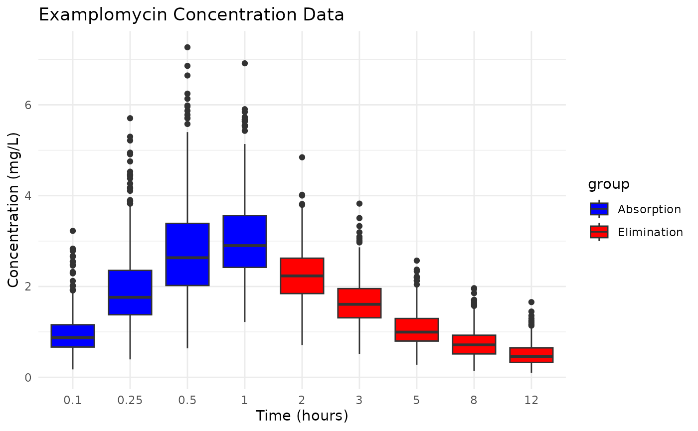
Model Specification
Defining the Pharmacokinetic Model
We’ll use a two-compartment model with first-order absorption. We use a solved model approach for simplicity. The model parameters include:
Creating the Prediction Function
The prediction function is crucial for the admr package.
It: - Constructs the event table for dosing and sampling - Solves the
RxODE model - Returns predicted concentrations in the required
format
rxode2::rxSetSilentErr(1)## [1] TRUE
predder <- function(time, theta_i, dose = 100) {
    n_individuals <- nrow(theta_i)

    if (is.null(n_individuals)) {
      n_individuals <- 1
    }

    # Create event table
    ev <- eventTable(amount.units="mg", time.units="hours")
    ev$add.dosing(dose = dose, nbr.doses = 1, start.time = 0)
    ev$add.sampling(time)

    # Solve model
    out <- rxSolve(rxModel, params = theta_i, events = ev, cores = 0)

    # Format output
    cp_matrix <- matrix(out$cp, nrow = n_individuals, ncol = length(time),
                        byrow = TRUE)

    return(cp_matrix)
}
Since both datasets come from the same study design, we can use the
same prediction function for both datasets. However, if the datasets had
different dosing regimens or other characteristics, you would need to
define separate prediction functions for each dataset. This can be done
by creating multiple genopts objects, each with its own
prediction function.
Model Fitting
Setting Up Model Options
The genopts function creates an options object that
controls the model fitting process:
opts1 <- genopts(
  time = c(.1, .25, .5, 1),  # Observation times
  p = list(
    beta = c(cl = 5, v1 = 10, v2 = 30, q = 10, ka = 1),  # Population parameters
    Omega = matrix(c(0.09, 0, 0, 0, 0,
                    0, 0.09, 0, 0, 0,
                    0, 0, 0.09, 0, 0,
                    0, 0, 0, 0.09, 0,
                    0, 0, 0, 0, 0.09), nrow = 5, ncol = 5),  # Random effects
    Sigma_prop = 0.04  # Proportional error
  ),
  nsim = 10000,  # Number of Monte Carlo samples
  n = 500,      # Number of individuals
  fo_appr = FALSE,  # Disable first-order approximation
  omega_expansion = 1,  # Omega expansion factor
  f = predder    # Prediction function
)


opts2 <- genopts(
  time = c(2, 3, 5, 8, 12),  # Observation times
  p = list(
    beta = c(cl = 5, v1 = 10, v2 = 30, q = 10, ka = 1),  # Population parameters
    Omega = matrix(c(0.09, 0, 0, 0, 0,
                    0, 0.09, 0, 0, 0,
                    0, 0, 0.09, 0, 0,
                    0, 0, 0, 0.09, 0,
                    0, 0, 0, 0, 0.09), nrow = 5, ncol = 5),  # Random effects
    Sigma_prop = 0.04  # Proportional error
  ),
  nsim = 10000,  # Number of Monte Carlo samples
  n = 500,      # Number of individuals
  fo_appr = FALSE,  # Disable first-order approximation
  omega_expansion = 1,  # Omega expansion factor
  f = predder    # Prediction function
)
The difference between opts1 and opts2 is
the observation times specified in the time argument.
Fitting the Model
Before fitting the model, ensure the opts objects and
aggregated datasets are organized into lists. The fitIRMC
function fits the model using the IR-MC algorithm:
opts <- list(opts1,opts2)
examplomycin_aggregated <- list(examplomycin_aggregated1, examplomycin_aggregated2)

fit.admr <- fitIRMC(
  opts = opts,
  obs = examplomycin_aggregated,
  chains = 2,  # Number of parallel chains
  maxiter = 2000,  # Maximum iterations
  single_dataframe = FALSE,  # Use separate data frames for each dataset
  use_grad = TRUE
)
## Chain 1:
## Iter | NLL and Parameters (11 values)
## --------------------------------------------------------------------------------
## 1: -1790.659 1.609 2.303 3.401 2.303 0.000 -2.408 -2.408 -2.408 -2.408 -2.408 -3.219
##
## ### Wide Search Phase ###
## 2: -1796.419 1.603 2.326 3.393 2.286 0.032 -2.265 -2.052 -2.306 -2.267 -2.565 -3.235
## 3: -1796.484 1.602 2.305 3.401 2.284 0.013 -2.271 -2.105 -2.324 -2.308 -2.509 -3.235
## 4: -1796.484 1.602 2.305 3.401 2.284 0.013 -2.271 -2.105 -2.325 -2.307 -2.509 -3.235
## 5: -1796.484 1.602 2.305 3.400 2.284 0.013 -2.271 -2.105 -2.325 -2.307 -2.509 -3.235
## 6: -1796.484 1.602 2.305 3.400 2.284 0.013 -2.271 -2.105 -2.325 -2.307 -2.509 -3.235
## 7: -1796.484 1.602 2.305 3.400 2.284 0.013 -2.271 -2.105 -2.325 -2.307 -2.509 -3.235
## 8: -1796.484 1.602 2.305 3.400 2.284 0.013 -2.271 -2.105 -2.325 -2.307 -2.509 -3.235
## 9: -1796.484 1.602 2.305 3.400 2.284 0.013 -2.271 -2.105 -2.325 -2.306 -2.509 -3.235
## 10: -1796.484 1.602 2.305 3.400 2.284 0.013 -2.271 -2.105 -2.325 -2.306 -2.509 -3.235
## 11: -1796.484 1.602 2.305 3.400 2.284 0.014 -2.271 -2.105 -2.326 -2.305 -2.509 -3.235
## 12: -1796.484 1.602 2.305 3.400 2.284 0.014 -2.271 -2.105 -2.326 -2.305 -2.509 -3.235
## 13: -1796.484 1.602 2.307 3.399 2.285 0.016 -2.271 -2.107 -2.330 -2.299 -2.507 -3.235
## 14: -1796.484 1.602 2.307 3.399 2.285 0.016 -2.271 -2.107 -2.330 -2.299 -2.507 -3.235
## Phase Wide Search Phase converged at iteration 14.
##
## ### Focussed Search Phase ###
## 15: -1796.484 1.602 2.307 3.399 2.285 0.016 -2.271 -2.107 -2.330 -2.299 -2.507 -3.235
## 16: -1796.484 1.602 2.307 3.399 2.285 0.016 -2.271 -2.107 -2.330 -2.299 -2.507 -3.235
## Phase Focussed Search Phase converged at iteration 16.
##
## ### Fine-Tuning Phase ###
## 17: -1796.484 1.602 2.307 3.399 2.285 0.016 -2.271 -2.107 -2.330 -2.299 -2.507 -3.235
## 18: -1796.484 1.602 2.307 3.399 2.285 0.016 -2.271 -2.107 -2.330 -2.299 -2.507 -3.235
## Phase Fine-Tuning Phase converged at iteration 18.
##
## ### Precision Phase ###
## 19: -1796.484 1.602 2.307 3.399 2.285 0.016 -2.271 -2.107 -2.330 -2.299 -2.507 -3.235
## 20: -1796.484 1.602 2.307 3.399 2.285 0.016 -2.271 -2.107 -2.330 -2.299 -2.507 -3.235
## 21: -1796.484 1.602 2.307 3.399 2.285 0.016 -2.271 -2.107 -2.330 -2.299 -2.507 -3.235
## 22: -1796.484 1.602 2.307 3.399 2.285 0.016 -2.271 -2.107 -2.330 -2.299 -2.507 -3.235
## 23: -1796.484 1.602 2.307 3.399 2.285 0.016 -2.271 -2.107 -2.330 -2.299 -2.507 -3.235
## Phase Precision Phase converged at iteration 23.
##
## Chain 1 Complete: Final NLL = -1796.484, Time Elapsed = 25.20 seconds
##
## Phase Wide Search Phase converged at iteration 11.
## Phase Focussed Search Phase converged at iteration 17.
## Phase Fine-Tuning Phase converged at iteration 19.
## Phase Precision Phase converged at iteration 24.
##
## Chain 2 Complete: Final NLL = -1796.483, Time Elapsed = 27.70 seconds
## Model Diagnostics
Basic Diagnostics
The print method provides a summary of the model
fit:
print(fit.admr)## -- FitIRMC Summary --
##
## -- Objective Function and Information Criteria --
## Log-likelihood: -1796.4840
## AIC: 3603.97
## BIC: 3729.69
## Condition#(Cov): 165.59
## Condition#(Cor): 271.86
##
## -- Timing Information --
## Best Chain: 25.2037 seconds
## All Chains: 52.9096 seconds
## Covariance: 35.7961 seconds
## Elapsed: 88.71 seconds
##
## -- Population Parameters --
## # A tibble: 6 × 6
## Parameter Est. SE `%RSE` `Back-transformed(95%CI)` `BSV(CV%)`
## <chr> <dbl> <dbl> <dbl> <chr> <dbl>
## 1 cl 1.60 0.0156 0.971 4.96 (4.81, 5.12) 32.1
## 2 v1 2.31 0.0945 4.10 10.03 (8.33, 12.07) 34.9
## 3 v2 3.40 0.0439 1.29 29.97 (27.50, 32.67) 31.3
## 4 q 2.28 0.0206 0.903 9.82 (9.43, 10.22) 31.6
## 5 ka 0.0136 0.0898 661. 1.01 (0.85, 1.21) 28.5
## 6 Residual Error 0.0394 NA NA 0.0394 NA
##
## -- Iteration Diagnostics --
## Iter | NLL and Parameters
## --------------------------------------------------------------------------------
## 1: -1790.659 1.609 2.303 3.401 2.303 0.000 -2.408 -2.408 -2.408 -2.408 -2.408 -3.219
## 2: -1796.419 1.603 2.326 3.393 2.286 0.032 -2.265 -2.052 -2.306 -2.267 -2.565 -3.235
## 3: -1796.484 1.602 2.305 3.401 2.284 0.013 -2.271 -2.105 -2.324 -2.308 -2.509 -3.235
## 4: -1796.484 1.602 2.305 3.401 2.284 0.013 -2.271 -2.105 -2.325 -2.307 -2.509 -3.235
## 5: -1796.484 1.602 2.305 3.400 2.284 0.013 -2.271 -2.105 -2.325 -2.307 -2.509 -3.235
## ... (omitted iterations) ...
## 19: -1796.484 1.602 2.307 3.399 2.285 0.016 -2.271 -2.107 -2.330 -2.299 -2.507 -3.235
## 20: -1796.484 1.602 2.307 3.399 2.285 0.016 -2.271 -2.107 -2.330 -2.299 -2.507 -3.235
## 21: -1796.484 1.602 2.307 3.399 2.285 0.016 -2.271 -2.107 -2.330 -2.299 -2.507 -3.235
## 22: -1796.484 1.602 2.307 3.399 2.285 0.016 -2.271 -2.107 -2.330 -2.299 -2.507 -3.235
## 23: -1796.484 1.602 2.307 3.399 2.285 0.016 -2.271 -2.107 -2.330 -2.299 -2.507 -3.235Convergence Assessment
The plot method visualizes the convergence of the model
fit:
plot(fit.admr)
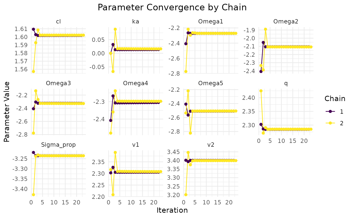

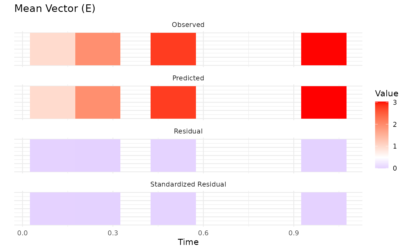
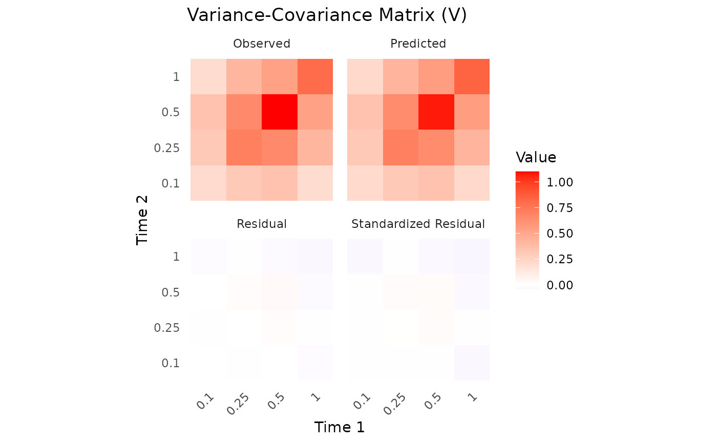
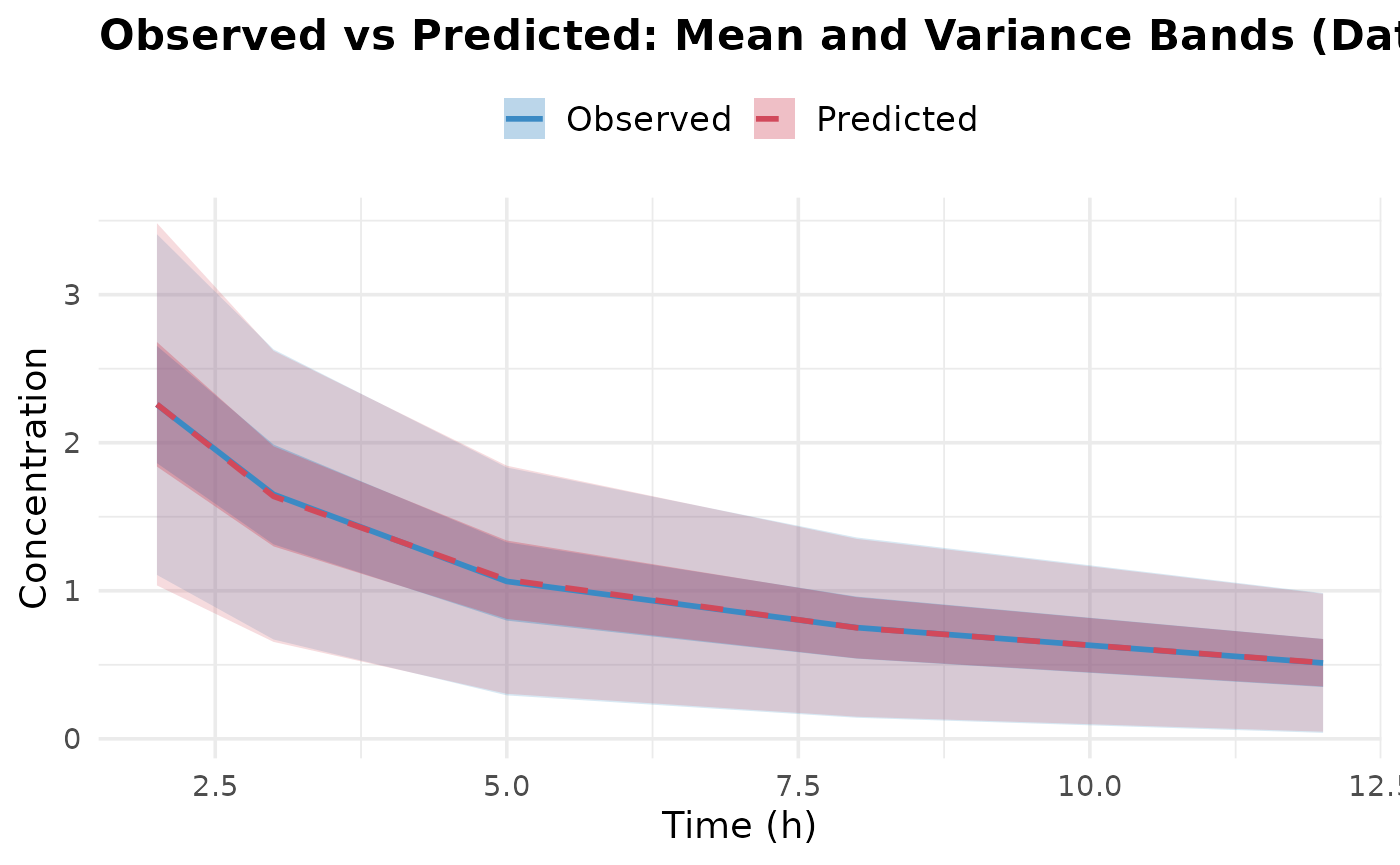
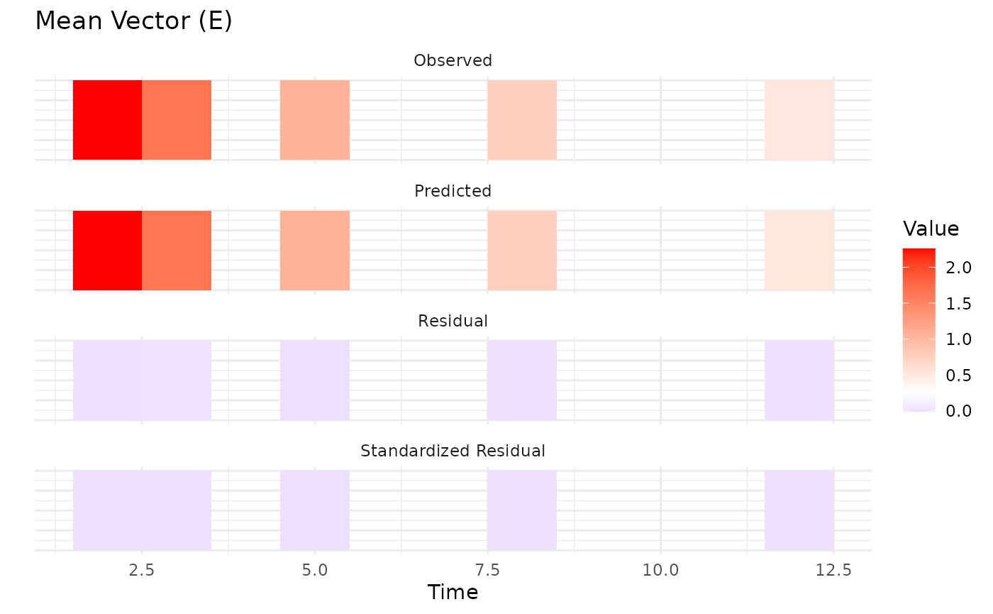
 Upon inspection of the convergence plots, you should look for: good
chain convergence, overlapping predicted and observed summary plots, and
similar final observed vs predicted matrices for mean and covariance. We
observe that the chains converge well, and the predicted means and
covariances align closely with the observed data.
Upon inspection of the convergence plots, you should look for: good
chain convergence, overlapping predicted and observed summary plots, and
similar final observed vs predicted matrices for mean and covariance. We
observe that the chains converge well, and the predicted means and
covariances align closely with the observed data.
Parameter Estimates
Let’s examine the parameter estimates and the true values used in the simulation. We expect to be close to the true values, although, like discussed earlier, the estimates may be less precise due to the reduced information content from splitting the data:
# True parameter values
params.true <- list(
  beta = c(cl = 5, v1 = 10, v2 = 30, q = 10, ka = 1),
  Omega = diag(rep(0.09, 5)),
  Sigma_prop = 0.04
)
cat("True parameter values:\n")
## True parameter values:
print(params.true)## $beta
## cl v1 v2 q ka
## 5 10 30 10 1
##
## $Omega
## [,1] [,2] [,3] [,4] [,5]
## [1,] 0.09 0.00 0.00 0.00 0.00
## [2,] 0.00 0.09 0.00 0.00 0.00
## [3,] 0.00 0.00 0.09 0.00 0.00
## [4,] 0.00 0.00 0.00 0.09 0.00
## [5,] 0.00 0.00 0.00 0.00 0.09
##
## $Sigma_prop
## [1] 0.04
# Extract parameter estimates
params <- fit.admr$transformed_params
cat("Final parameter estimates:\n")
## Final parameter estimates:
print(params)## $beta
## cl v1 v2 q ka
## 4.962068 10.029070 29.972972 9.819855 1.013666
##
## $Omega
## [,1] [,2] [,3] [,4] [,5]
## [1,] 0.1031986 0.0000000 0.00000000 0.00000000 0.0000000
## [2,] 0.0000000 0.1218244 0.00000000 0.00000000 0.0000000
## [3,] 0.0000000 0.0000000 0.09771018 0.00000000 0.0000000
## [4,] 0.0000000 0.0000000 0.00000000 0.09971726 0.0000000
## [5,] 0.0000000 0.0000000 0.00000000 0.00000000 0.0813899
##
## $Sigma_prop
## [1] 0.03935017We observe that the parameter estimates are reasonably close to the
true values, especially considering the reduced information content from
splitting the data into two groups. There are some deviations,
particularly in the estimates of q and the random effect of
v1, which may be attributed to the lack of early timepoint
data in the second dataset. Let’s also visualize the dynamics of the
estimated model together with the true model through a dosing
simulation. ## Advanced Features
Creating a dosing plot
To visualize the dosing regimen and predicted concentrations, we can
create a dosing plot. This helps in understanding the pharmacokinetic
profile of the drug over time. This can be done using the
nlmixr2-universe. First, we need to define the model in
nlmixr2 syntax and then simulate the dosing regimen of both
the estimated and true models.
Click here
params.true <- list(
  beta = c(cl = 5, v1 = 10, v2 = 30, q = 10, ka = 1),
  Omega = diag(rep(0.09, 5)),
  Sigma_prop = 0.04
)
params <- fit.admr$transformed_params

rxModel_true <- function(){
  ini({
    cl <- params.true$beta["cl"]  # Clearance
    v1 <- params.true$beta["v1"]  # Volume of central compartment
    v2 <- params.true$beta["v2"] # Volume of peripheral compartment
    q <- params.true$beta["q"]    # Inter-compartmental clearance
    ka <- params.true$beta["ka"]   # Absorption rate constant

    eta_cl ~ params.true$Omega[1,1]
    eta_v1 ~ params.true$Omega[2,2]
    eta_v2 ~ params.true$Omega[3,3]
    eta_q ~ params.true$Omega[4,4]
    eta_ka ~ params.true$Omega[5,5]
  })
  model({
    cl <- cl * exp(eta_cl)
    v1 <- v1 * exp(eta_v1)
    v2 <- v2 * exp(eta_v2)
    q <- q * exp(eta_q)
    ka <- ka * exp(eta_ka)
    cp = linCmt(cl, v1, v2, q, ka)
  })
}

rxModel_multiple <- function(){
  ini({
    cl <- params$beta["cl"]  # Clearance
    v1 <- params$beta["v1"]  # Volume of central compartment
    v2 <- params$beta["v2"] # Volume of peripheral compartment
    q <- params$beta["q"]    # Inter-compartmental clearance
    ka <- params$beta["ka"]   # Absorption rate constant

    eta_cl ~ params$Omega[1,1]
    eta_v1 ~ params$Omega[2,2]
    eta_v2 ~ params$Omega[3,3]
    eta_q ~ params$Omega[4,4]
    eta_ka ~ params$Omega[5,5]
  })
  model({
    cl <- cl * exp(eta_cl)
    v1 <- v1 * exp(eta_v1)
    v2 <- v2 * exp(eta_v2)
    q <- q * exp(eta_q)
    ka <- ka * exp(eta_ka)
    cp = linCmt(cl, v1, v2, q, ka)
  })
}

rxModel_true <- rxode2(rxModel_true())
rxModel_true <- rxModel_true$simulationModel
rxModel_multiple <- rxode2(rxModel_multiple())
rxModel_multiple <- rxModel_multiple$simulationModel
Now that we have defined both models, we can simulate the dosing regimen and plot the results:
time_points <- seq(0, 12, by = 0.05)  # Dense time points for smooth curves
ev <- eventTable(amount.units="mg", time.units="hours")
ev$add.dosing(dose = 100, nbr.doses = 2, dosing.interval = 6)
ev$add.sampling(time_points)

sim_true <- rxSolve(rxModel_true, events = ev, cores = 0, nSub = 10000)
sim_multiple <- rxSolve(rxModel_multiple, events = ev, cores = 0, nSub = 10000)

# Combine the confidence intervals with a label for the model
ci_true <- as.data.frame(confint(sim_true, "cp", level=0.95)) %>%
  mutate(Model = "True parameters")
## summarizing data...done
ci_covar <- as.data.frame(confint(sim_multiple, "cp", level=0.95)) %>%
  mutate(Model = "Estimated model")
## summarizing data...done
# Bind them together
ci_all <- bind_rows(ci_true, ci_covar) %>%
  mutate(
    p1 = as.numeric(as.character(p1)),
    Percentile = factor(Percentile, levels = unique(Percentile[order(p1)]))
  )

# Plot both models
ggplot(ci_all, aes(x = time, group = interaction(Model, Percentile))) +
  geom_ribbon(aes(ymin = p2.5, ymax = p97.5, fill = Model),
              alpha = 0.2, colour = NA) +
  geom_line(aes(y = p50, colour = Model), size = 0.8) +
  labs(
    title = "Central Concentration Simulations",
    x = "Time",
    y = "Central Concentration (mg/L)"
  ) +
  theme_bw(base_size = 14) +
  scale_colour_manual(values = c("True parameters" = "blue",
                                 "Estimated model" = "red")) +
  scale_fill_manual(values = c("True parameters" = "blue",
                               "Estimated model" = "red"))
## Warning: Using `size` aesthetic for lines was deprecated in ggplot2 3.4.0.
## ℹ Please use `linewidth` instead.
## This warning is displayed once per session.
## Call `lifecycle::last_lifecycle_warnings()` to see where this warning was
## generated.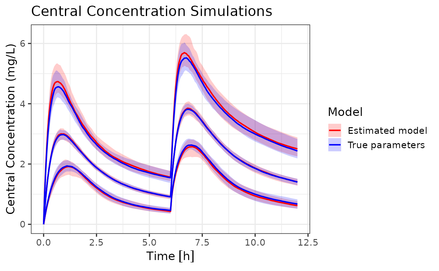
The combined dataset model (red) closely follows the true parameter model (blue). The median line of the estimated model almost perfectly overlaps with the true model, indicating that the estimated model. However, the estimated model does show slightly wider population intervals. In this scenario this isn’t very problematic, since a wider range still captures the true dynamics. In case of dose optimization, this results in a more conservative dose recommendation. However, in other scenarios, this could lead to over- or under-prediction of certain percentiles. The estimation error is expected due to the reduced information content in variance-only data.
Best Practices
So to conclude, here are some best practices when using the
admr package for aggregate data modeling:
-
Data Preparation:
- Always check your data for missing values and outliers
- Ensure time points are consistent across subjects
- Consider the impact of dosing events on your analysis
-
Model Specification:
- Start with a simple model and gradually add complexity
- Use meaningful initial values for parameters
- Consider parameter transformations for better estimation
-
Model Fitting:
- Use multiple chains to improve optimization
- Monitor convergence carefully
- Check parameter estimates for biological plausibility
-
Diagnostics:
- Always examine convergence plots
- Validate model predictions against observed data
For more information, see the package documentation and other vignettes.